How to Convert a Jupyter Notebook to PDF (Without LaTeX Errors)
Jupyter's PDF export failing with xelatex or pandoc errors? Convert your notebook to PDF via HTML, nbconvert's webpdf or online, with code hidden or shown.

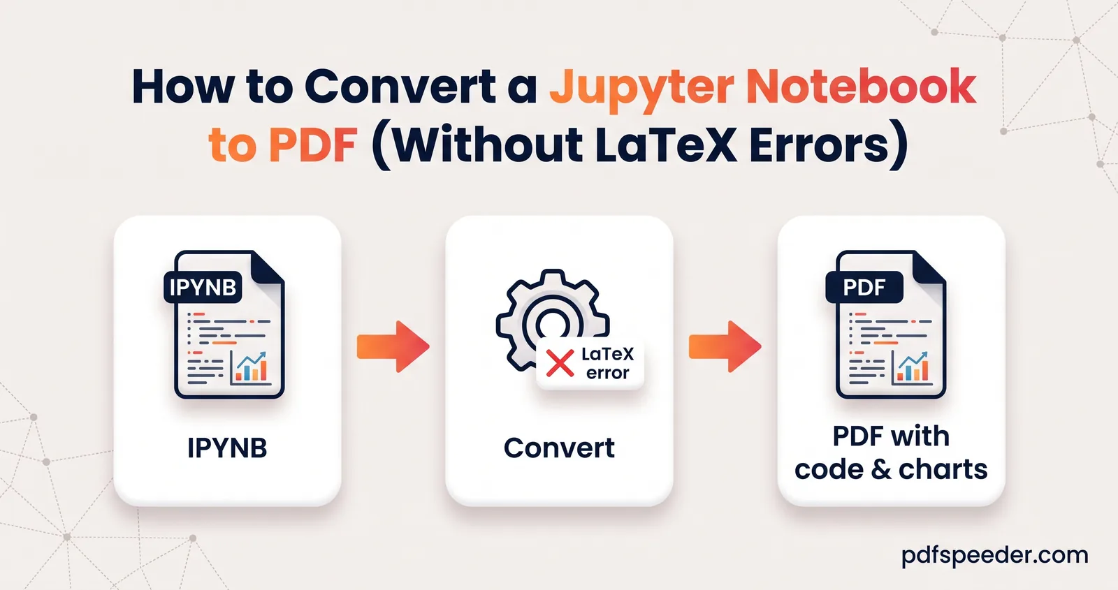
Jupyter's built-in PDF export goes through pandoc and LaTeX, so on most computers it stops with "Pandoc wasn't found" or "xelatex not found on PATH". You don't need to install LaTeX to convert a Jupyter notebook to PDF: export it as HTML and print that from your browser, use nbconvert's Chromium-based webpdf exporter, or upload the .ipynb file to an online converter that never runs your code. Below, each route is explained, along with the settings that decide whether your equations, long code lines and outputs survive.
On this page
Why Jupyter's PDF export often fails
When you choose PDF in Jupyter's export menu, nbconvert doesn't print the page you see. It rewrites the notebook as a LaTeX document, using pandoc to turn your Markdown cells into LaTeX, then runs XeLaTeX to typeset it. Neither pandoc nor a TeX distribution comes with Jupyter, so the export stops at the first missing piece. In JupyterLab or Notebook, that appears as a "500 : Internal Server Error" page with a line starting "nbconvert failed:".
| The message you see | What's missing | Quickest way round it |
|---|---|---|
| Pandoc wasn't found | pandoc, which converts Markdown cells to LaTeX | Install pandoc, or skip LaTeX entirely |
| xelatex not found on PATH | A TeX distribution that includes XeLaTeX | Install TeX, or skip LaTeX entirely |
| ! LaTeX Error: File `adjustbox.sty' not found | A LaTeX package the template uses | Install that package or a fuller TeX setup |
| No suitable chromium executable found on the system | Chromium, for the webpdf exporter | Add --allow-chromium-download |
In a test on a sample notebook with nbconvert 7.17 and neither tool installed, --to pdf failed at the pandoc step before it ever reached LaTeX. On a machine without TeX, installing pandoc simply moves you on to the xelatex error. That's why most people are better off with one of the three routes below, which don't touch LaTeX at all.
Option 1: Export to HTML, then print to PDF
Every Jupyter install can export HTML, and every browser can save a page as a PDF, so this route works almost anywhere:
- Save the notebook, then choose File > Save and Export Notebook As > HTML in JupyterLab or Notebook 7. In the classic Notebook it's File > Download as > HTML (.html).
- Open the HTML file in Chrome or Edge while you're online. The page loads MathJax from the internet to typeset your equations, so give it a few seconds.
- Press Ctrl+P (Cmd+P on a Mac) and set the destination to Save as PDF.
- Under More settings, tick Background graphics so code cells keep their grey shading, and pick your paper size.
- Select Save.
The result keeps selectable text, syntax colours and properly typeset maths. Its weak spot is width. Browsers don't wrap code, so anything wider than the page gets cut off: in our test, only the first 80 or so characters of a 241-character line of code made it onto an A4 page.
Wide DataFrames lose their right-hand columns in the same way. Lowering Scale to 70-80% or switching to landscape helps, but breaking long lines in the notebook itself is the reliable fix. You also don't get bookmarks, which matters for a 40-page report.
Working in Google Colab? File > Print sends the notebook straight to the same print dialog, with the same width limits. Our guide to printing anything to PDF covers paper size and margin fixes in more detail.
Option 2: Use nbconvert from the command line
If you're comfortable in a terminal, nbconvert's webpdf exporter renders the notebook as HTML and prints it with headless Chromium, no LaTeX involved:
pip install "nbconvert[webpdf]"
jupyter nbconvert --to webpdf --allow-chromium-download analysis.ipynb
The flag lets nbconvert download a copy of Chromium the first time, and later runs reuse it. Your PDF lands next to the notebook as analysis.pdf. Here's how the main commands compare:
| Command | Needs | What you get |
|---|---|---|
jupyter nbconvert --to webpdf analysis.ipynb |
Playwright and Chromium | A PDF that looks like JupyterLab |
jupyter nbconvert --to pdf analysis.ipynb |
pandoc plus TeX with XeLaTeX | A LaTeX-typeset, article-style PDF |
jupyter nbconvert --to html analysis.ipynb |
Nothing extra | An HTML file to print yourself (Option 1) |
Three flags work with all of them. --no-input hides the code cells and their prompts, leaving a code-free report. --no-prompt keeps the code but drops the In [ ] and Out [ ] labels. --execute runs the notebook from top to bottom before converting, which needs the notebook's kernel and packages on that machine.
If you need the LaTeX look, for a thesis appendix, say, the nbconvert installation guide recommends TeX Live on Linux, MacTeX on a Mac and a Windows TeX distribution such as MiKTeX, plus pandoc. On Debian or Ubuntu, its suggested command is sudo apt-get install texlive-xetex texlive-fonts-recommended texlive-plain-generic.
Option 3: Convert a Jupyter notebook to PDF online
When you can't install anything, on a lab computer or a phone, say, our IPYNB to PDF converter does the rendering for you. It uses Jupyter's own nbconvert to lay out the notebook and a real Chromium browser to print it, and it only reads the file: no code is ever executed.
- Run and save first. Because nothing is executed, the PDF shows only the outputs saved in the file. A cell you never ran prints as code with an empty "In [ ]" and no result.
- Get the .ipynb file. From JupyterLab, it's the file itself. To convert a Colab notebook to PDF, choose File > Download > Download .ipynb in Colab first.
- Add your notebooks. Drop one or several .ipynb files onto the page.
- Pick what to include. Code cells, cell outputs, In [ ]/Out [ ] prompts, wrapping of long lines and bookmarks from headings are all on by default. You can also choose A4, US Letter, US Legal or A3, portrait or landscape, four margin sizes and page numbers.
- Convert and download. Preview the PDF on the page, then download it. With several notebooks, you get a ZIP, or tick Combine all into one PDF before converting.
Notebooks of up to 60 MB are uploaded over an encrypted connection and deleted from our server automatically within 2 hours. Each notebook counts as one task in the free daily allowance: 2 tasks a day without an account, 3 with a free account, reset at 00:00 UTC (05:30 IST).
In our test, this produced a Jupyter notebook to PDF with outputs intact: the matplotlib chart, the DataFrame table and an error traceback all appeared, the long line wrapped instead of being cut off, and every Markdown heading became a bookmark. One honest limit: because the converter works offline, LaTeX equations appear as their source text, such as $\bar{x} = \frac{1}{n}\sum x_i$, rather than typeset. For an equation-heavy notebook, use Option 1 or 2.
Hide code, keep outputs: what to include
The right settings depend on who's reading. A good starting point:
| Who's reading | Code cells | Outputs | Prompts |
|---|---|---|---|
| A professor or grader | Show | Show | Show, so they can point to "In [12]" |
| A manager or client | Hide | Show | Hide |
| A colleague reusing your method | Show | Hide or show | Hide |
A few checks before you convert make the PDF look deliberate rather than accidental:
- Run everything in order. Use Kernel > Restart Kernel and Run All Cells in JupyterLab, or Runtime > Run all in Colab, then save. Prompts that run In [1], In [2], In [3] down the page show the notebook works from a clean start; a stray In [47] above In [3] suggests it doesn't.
- Clear errors you don't mean to show. A traceback is an output, so it stays in the PDF even with code hidden.
- Expect empty cells to vanish. With code hidden, a cell that produced nothing disappears, though its Markdown heading stays. If hiding code leaves a blank last page, as it did once in our tests, Delete PDF Pages removes it.
- Save interactive charts as images. Widgets and interactive plots rely on JavaScript, so a static PDF may show them blank or as a line of placeholder text. A static image (matplotlib, or the library's own image export) always prints.
- Keep Wrap long lines on. Without it, long code and output lines are cut off at the margin, just as in the browser route.
Need a cover page or a signed declaration in front of the notebook? Convert it, then put the pages together with Merge PDF, which runs in your browser and also counts as one task. For other file types, our guide to converting documents to PDF matches each format to the right method.
Ready to try it? Restart and run your notebook, save it, then drop the .ipynb file into IPYNB to PDF and check the preview before you download.
Frequently asked questions
Why does Jupyter say "xelatex not found on PATH"?
Jupyter's PDF export compiles the notebook with XeLaTeX, which isn't installed with Jupyter. Install a TeX distribution and pandoc, or skip LaTeX by exporting HTML and printing it, using nbconvert's webpdf exporter, or converting the .ipynb file online.
Do I need to run my notebook before converting it?
Yes. Converters print the outputs saved in the .ipynb file, and ours never executes code, so restart the kernel, run all cells and save before converting.
How do I convert a Colab notebook to PDF?
In Colab, choose File > Download > Download .ipynb, then convert that file with IPYNB to PDF. For a quick copy, File > Print in Colab saves the page through your browser's print dialog.
Can I hide the code and keep only the outputs?
Yes. Untick Include code cells in IPYNB to PDF, or add --no-input to an nbconvert command, and the PDF shows Markdown and outputs only.
Will my LaTeX equations show up in the PDF?
In the HTML route, your browser typesets them as long as you open the file while online. Our IPYNB to PDF converter works offline and shows equations as their LaTeX source text.